GEOG 868: Jen and Barry's Site Selection

In Lesson 4 of GEOG 868 I completed a site selection using PostGIS.

Project Brief #

For this project I was supplied with 4 shapefiles that describe a (slightly made up) chunk of the state of Pennsylvania, USA – counties, cities, roads, and some recreation areas. Jen and Barry were looking to open an ice cream business, and had the following criteria for locating a suitable site:

1. Greater than 500 farms for milk production
2. A labor pool of at least 25,000 individuals between the ages of 18 and 64 years
3. A low crime index (less than or equal to 0.02)
4. A population of less than 150 individuals per square mile
5. Located near a university or college
6. At least one recreation area within 10 miles
7. Interstate within 20 miles

My approach for tackling this looked roughly like:

• visidata to inspect attribute tables of shapefiles
• psql to create a fresh database and schema
• ogr2ogr to load shapefiles into PostGIS
• pgAdmin to craft the SQL for site selection criteria
• QGIS to make a nice map

When it came to the pgAdmin part, I followed the workflow from the tips in the project brief, which was to work from large to small. Narrow down based on counties, then cities, then proximity to interstates (within 20 miles), then proximity to recreation areas (within 10 miles).

Initial inspection of data #

Using visidata I perused the attribute tables of the shapefiles provided. I was looking to see which fields would cover the non-spatial criteria. I determined that the counties shapefile covered criteria 1, 2 and 4; the cities shapefile covered criteria 3 and 5; and the interstates shapefile covered criteria 7. For criteria 6, the proximity to a recreation area, there was no criteria to be filtered on before addressing the spatial aspect.

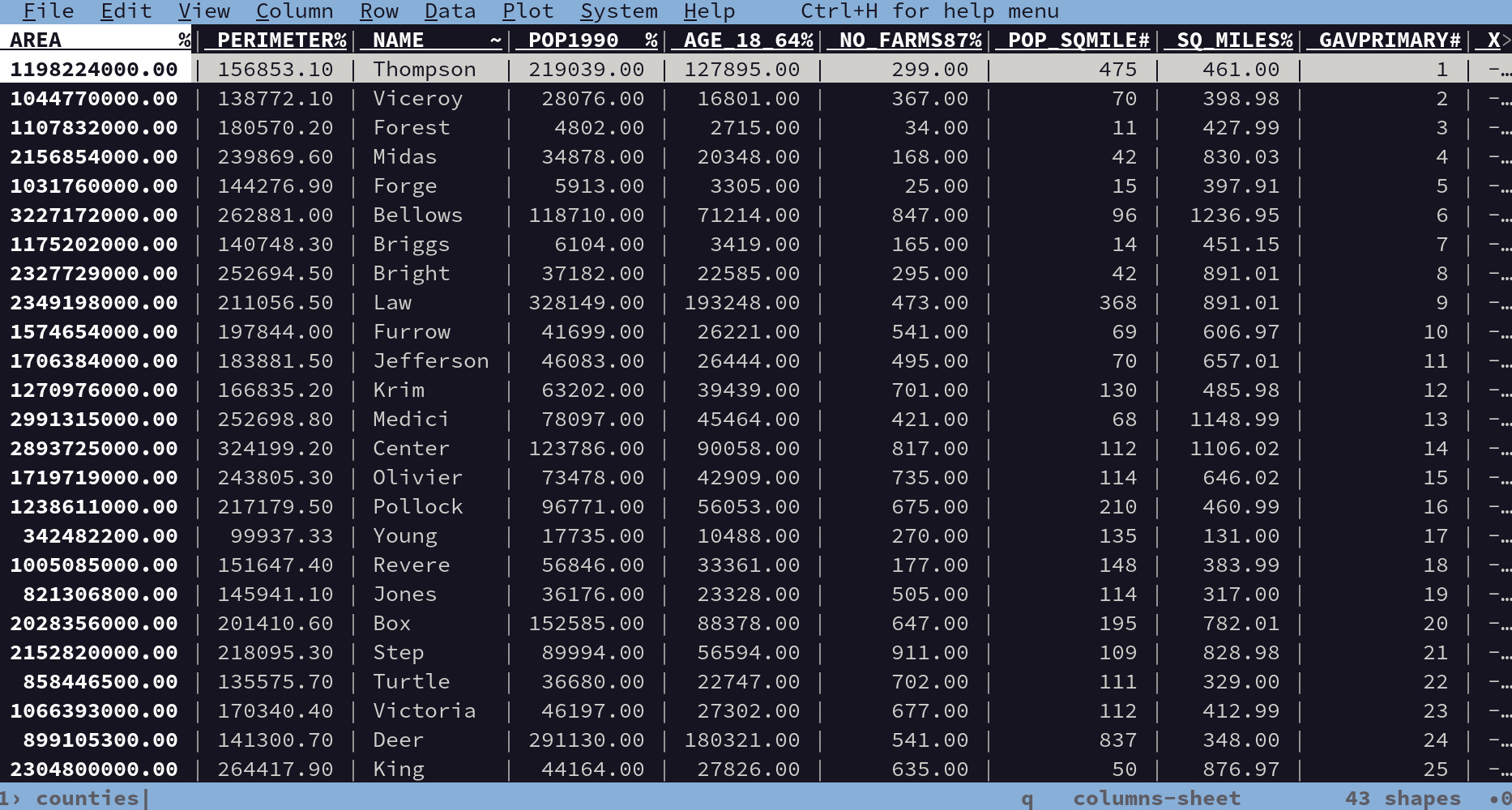
The counties shapefile attribute table in visidata

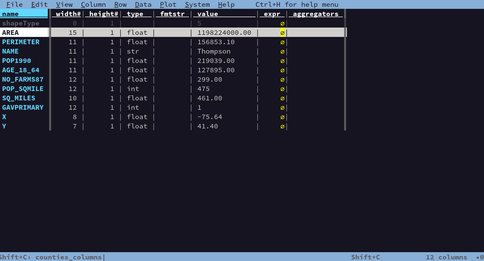
The fields in the counties shapefile

ER diagram #

After the initial inspection of the data it became apparent I didn’t have any need to sketch up an ER diagram, as there were no fields to join anything on! It was all going to be spatial joins.

Creating a fresh database and schema #

During the Lesson 4 exercises I was still working with the same data from Lesson 3, so I hadn’t yet created a new database. I figured I may as well create one now to refresh my memory.

$ sudo systemctl start postgresql
$ sudo -u postgres psql

postgres=# CREATE DATABASE Lesson4db OWNER postgres;
CREATE DATABASE
postgres=# \q

$ pgcli -h localhost -u postgres -W -d Lesson4db
Password for postgres: 
Password for postgres: 
FATAL:  database "Lesson4db" does not exist

$ pgcli -h localhost -u postgres -W -d lesson4db
Password for postgres: 
postgres@localhost:lesson4db>

Huh? It seems that creating a database via psql lowercases whatever name you give your database… When creating a database via pgAdmin it respects uppercase letters. Anyway, I carried on:

postgres@localhost:lesson4db> CREATE EXTENSION postgis;
CREATE EXTENSION
Time: 0.426s

postgres@localhost:lesson4db> CREATE SCHEMA jen_barry_site
 AUTHORIZATION postgres;
CREATE SCHEMA
Time: 0.004s

With a fresh PostGIS-enabled database ready, the next step was to stick the data in it.

Loading shapefiles into PostGIS #

I loaded the shapefiles into PostGIS using ogr2ogr as follows:

$ ogr2ogr -f PostgreSQL PG:"host=localhost port=5432 dbname=lesson4db user=postgres password=......" -lco SCHEMA=jen_barry_site -nlt GEOMETRY -t_srs EPSG:4267 counties.shp 

$ ogr2ogr -f PostgreSQL PG:"host=localhost port=5432 dbname=lesson4db user=postgres password=......" -lco SCHEMA=jen_barry_site -nlt GEOMETRY -t_srs EPSG:4267 cities.shp 

$ ogr2ogr -f PostgreSQL PG:"host=localhost port=5432 dbname=lesson4db user=postgres password=......" -lco SCHEMA=jen_barry_site -nlt GEOMETRY -t_srs EPSG:4267 interstates.shp 

$ ogr2ogr -f PostgreSQL PG:"host=localhost port=5432 dbname=lesson4db user=postgres password=......" -lco SCHEMA=jen_barry_site -nlt GEOMETRY -t_srs EPSG:4267 recareas.shp 

(This time specifying the CRS with -t_srs, unlike before where I didn’t and it eventually came back to bite me like I suspected it would.)

That went smoothly, except for one minor hiccup which was handled automatically by ogr2ogr. The interstates shapefile had 2 fields with the same name, so the second one was automatically renamed – I was informed by this warning in the output from ogr2ogr:

Warning 1: Field 'INTERSTATE' already exists. Renaming it as 'interstate2'

I had loaded the shapefiles into QGIS before now but hadn’t seen any such warning, so I went back to check what was going on. QGIS appears to quietly handle this, without so much as a warning (not even hiding a note in the log messages panel). QGIS had added a _1 suffix to the second “INTERSTATE” field and carried on like nothing ever happened.

With a database full of data, it was time to do the site selection spatial analysis part.

Crafting SQL for site selection criteria #

I switched from the command line to the GUI and used pgAdmin to work through building the SQL queries. pgAdmin is definitely a better environment for developing an SQL query than the command line, as its much easier to make a minor change to a query and re-run it. Also I could more easily flip between reference data from the table I was working with and the query I was building.

First up I narrowed down the possible counties based on the non-spatial criteria with this query:

SELECT * FROM counties
WHERE 1=1
AND no_farms87 > 500
AND age_18_64 >= 25000
AND pop_sqmile < 150
;

Then I narrowed down the possible cities based on the non-spatial criteria with another query:

SELECT * FROM cities
WHERE 1=1
AND crime_inde <= 0.02
AND university = 1
;

This left me with 11 counties and 18 cities. However, the cities were not necessarily in the suitable counties as I had not yet joined up the data. Time for a spatial join. I created a view for the valid counties, and then incorporated that into my query for selecting cities:

CREATE VIEW jen_barry_site.vw_valid_counties
 AS
SELECT * FROM jen_barry_site.counties
WHERE 1=1
AND no_farms87 > 500
AND age_18_64 >= 25000
AND pop_sqmile < 150
;

ALTER TABLE jen_barry_site.vw_valid_counties
    OWNER TO postgres;

SELECT * FROM cities
CROSS JOIN vw_valid_counties
WHERE 1=1
AND cities.crime_inde <= 0.02
AND cities.university = 1
AND ST_Contains(vw_valid_counties.wkb_geometry, cities.wkb_geometry)
;

This narrowed the cities down to 9, which was the right number so far according to the notes in the project brief.

(The WHERE 1=1 clause I used is something a DBA taught me once, it makes it easier to toggle criteria in your query on and off with comments, because you don’t need to change the first AND to a WHERE if you want to toggle off the first criteria you added, which would have started with WHERE)

With my cities successfully narrowed down, I created a view to use in the next part:

CREATE VIEW jen_barry_site.vw_valid_cities
 AS
SELECT * FROM jen_barry_site.cities
CROSS JOIN jen_barry_site.vw_valid_counties
WHERE 1=1
AND cities.crime_inde <= 0.02
AND cities.university = 1
AND ST_Contains(vw_valid_counties.wkb_geometry, cities.wkb_geometry)
;

ALTER TABLE jen_barry_site.vw_valid_cities
    OWNER TO postgres;

ERROR: column "ogc_fid" specified more than once

oops!

As I had been using SELECT * FROM ... with no problems until now, I didn’t see this one coming, but it quickly made sense. I started listing out field names in my SELECT and spotted another 2 fields that would have raised the same error had I not renamed them like this:

CREATE VIEW jen_barry_site.vw_valid_cities
 AS
SELECT
  cities.ogc_fid AS ogc_fid_city,
  cities.name AS name_city,
  cities.population,
  cities.total_crim,
  cities.wkb_geometry AS geom_city,
  vw_valid_counties.ogc_fid AS ogc_fid_county,
  vw_valid_counties.name AS name_county,
  vw_valid_counties.pop1990,
  vw_valid_counties.age_18_64,
  vw_valid_counties.no_farms87,
  vw_valid_counties.pop_sqmile,
  vw_valid_counties.wkb_geometry AS geom_county
FROM jen_barry_site.cities
CROSS JOIN jen_barry_site.vw_valid_counties
WHERE 1=1
AND cities.crime_inde <= 0.02
AND cities.university = 1
AND ST_Contains(vw_valid_counties.wkb_geometry, cities.wkb_geometry)
;

ALTER TABLE jen_barry_site.vw_valid_cities
    OWNER TO postgres;

While renaming the fields that were present in both tables, it occurred to me all the fields could have done with better names, to at least make it clearer which were county-level and which were city-level since they were joined together into a new view now. I was also aware that I wasn’t selecting only strictly necessary data, but I was thinking “maybe I’ll incorporate it into some styling on my map later or something” so I kept a few extra fields in.

For the remaining criteria (proximity to an interstate and a recreation area) I created only 1 further view, rather than the 2 suggested by the project brief’s workflow suggestion.

For this view, I took the valid cities, and joined them with both the interstates and the recreation areas. That made for a “large” intermediary result set, at least in the context of this small dataset. Since this was a small dataset queries still completed in milliseconds, but I can imagine stacking up too many CROSS JOIN statements with larger datasets becoming troublesome…

As these particular spatial criteria involved distances, I needed to ensure I was using an appropriate CRS / SRID. Without delving too far into State Plane Projections I determined the 2 possible choices for Pennsylvania and selected the “South” one, which was EPSG:2272.

CREATE VIEW jen_barry_site.vw_site_selection_cities
 AS
SELECT DISTINCT
  vw_valid_cities.name_city,
  vw_valid_cities.geom_city
FROM jen_barry_site.vw_valid_cities
CROSS JOIN jen_barry_site.interstates
CROSS JOIN jen_barry_site.recareas
WHERE interstates.type = 'Interstate'
AND ST_DWithin(
      ST_Transform(vw_valid_cities.geom_city,2272),
      ST_Transform(interstates.wkb_geometry,2272),
      5280*20)  -- within 20 miles. 5280 feet x20.
AND ST_DWithin(
      ST_Transform(vw_valid_cities.geom_city,2272),
      ST_Transform(recareas.wkb_geometry,2272),
      5280*10)  -- within 10 miles. 5280 feet x10. 
;

ALTER TABLE jen_barry_site.vw_site_selection_cities
    OWNER TO postgres;

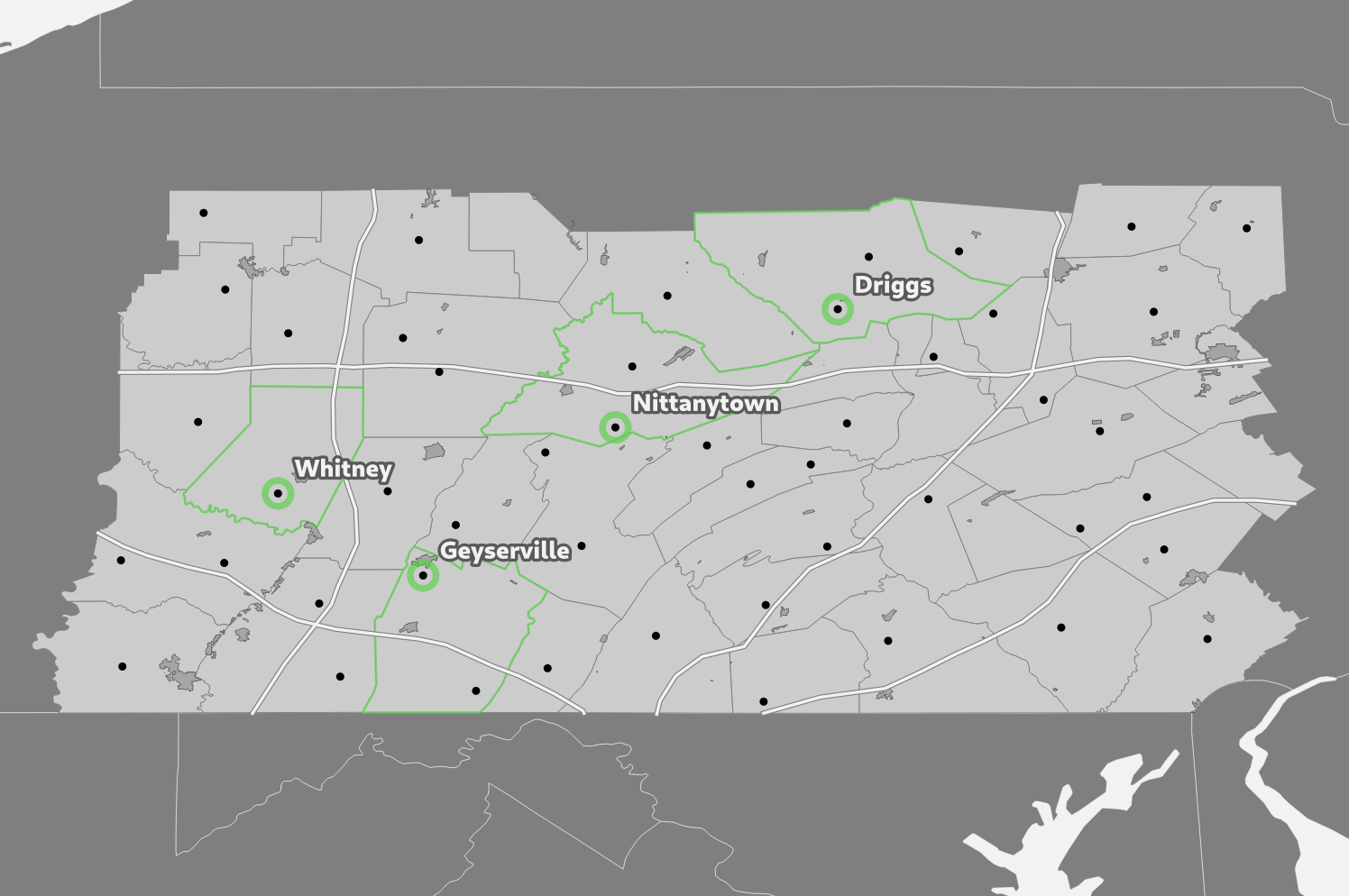
With that I had narrowed the suitable cities down to 4, just as the project brief prescribed. All that was left to do was make a map.

Make a nice map #

I thoroughly enjoy playing around with the cartography side of things. I easily spent over an hour altogether. First making a map I didn’t quite like, then coming back to it the next day and turning it (mostly) grayscale.

If I were to spend more time on it then typical map elements like a title, a legend, a scale bar, and a north arrow, would undoubtedly be the next things I add.

Header image from vecteezy